At the beginning of the year, I wrote a bunch of articles on the various tricks DOS played to overcome the tight memory limits of x86’s real mode. There was one question that came up and remained unanswered: what were the various “models” that the compilers of the day offered? Take a look at Borland Turbo C++’s code generation menu:

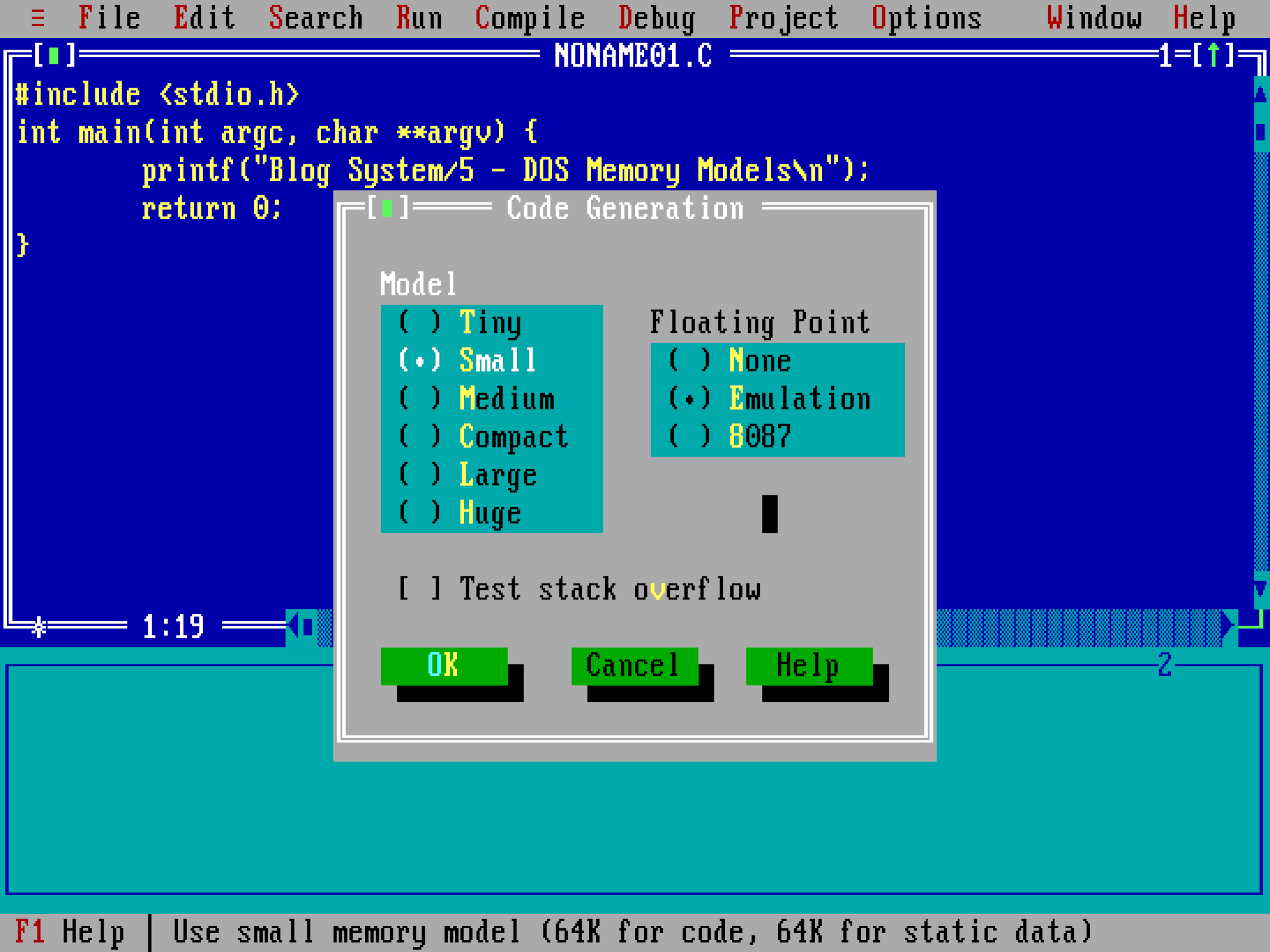
Tiny, small, medium, compact, large, huge… What did these options mean? What were their effects? And, more importantly… is any of that legacy relevant today in the world of 64-bit machines and gigabytes of RAM? To answer those questions, we must start with a brief review of the 8086 architecture and the binary formats supported by DOS.

8086 segmentation

In the 8086 architecture, which is the architecture that DOS targeted, memory references are composed of two parts: a 2-byte segment “identifier” and a 2-byte offset within the segment. These pairs are often expressed as segment:offset.

Segments are contiguous 64KB chunks of memory and are identified by their base address. To be able to address the full 1MB of memory that the 8086 supports, segments are offset from each other by 16 bytes. As you can deduce from this, segments overlap, which means that a specific physical memory position can be referenced by many segment/offset pairs.

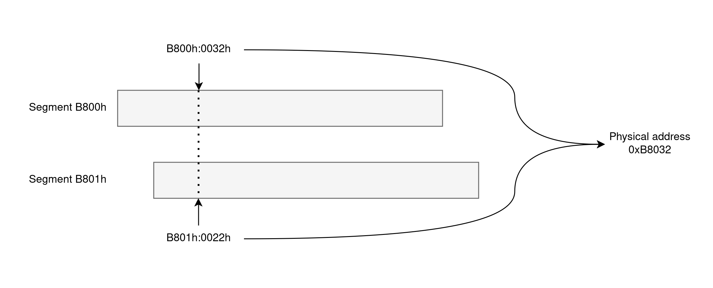
As an example, the segmented address B800h:0032h corresponds to the physical address B8032h computed via B800h * 10h + 0032h. While this pair is human-readable, that’s not how the machine-level instructions encode it. Instead, instructions rely on segment registers to specify the segment to access, and the 8086 supports four of these: CS (code segment), DS (data segment), ES (extra data segment), and SS (stack segment). Knowing this, accessing this sample memory position requires first loading B800h into DS and then referencing DS:0032h.

One of the reasons instructions rely on segment registers instead of segment identifiers on every memory access is efficiency: encoding the segment register to use requires only 2 bits (we have 4 segment registers in total) vs. the 2 bytes that would be necessary to store the segment base. More on this later.

COM files

COM files are the most trivial executable format you can think of: they contain raw machine code that can be placed at pretty much any memory location and executed without any sort of post-processing. There are no relocations, no shared libraries, no nothing to worry about: you can just blit the binary into memory and run it.

The way this works is by leveraging the 8086 segmented architecture: the COM image is loaded into any segment and always at offset 100h within that segment. All memory addresses within the COM image must be relative to this offset (which explains the ORG 100h you might have seen in the past), but the image doesn’t need to know which segment it is loaded into: the loader (DOS in our case, but COM files come from CP/M actually) sets CS, DS, ES, and SS to the exact same segment and transfers control to CS:100h.

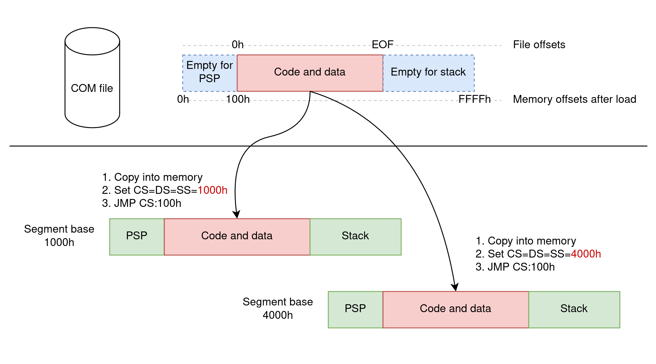
Magic! COM files are essentially PIE (Position Independent Executables) without requiring any sort of MMU or fancy memory management by the kernel.

Unfortunately, not everything is rosy. The problem with COM files is that they are limited in size: because they are loaded into one segment and segments are 64KB-long at most, the largest a COM file can be is 64KB (minus the 256 bytes reserved for the PSP at the front). This includes code and data, and 64KB isn’t much of either. Obviously, when the COM program is running, it has free reign over the processor and can access any memory outside of its single segment by resetting CS, DS, ES, and/or SS, but all memory management is left to the programmer.

EXE files

To resolve the limitations of COM files in DOS, Microsoft came up with a different executable format for DOS: the EXE file, also known as an MZ executable.

Compared to COM files, EXE files have some internal structure and are not bound by the 64KB limit: they can contain larger code and data blocks in them. But… how is that possible given that 8086 segments are still 64KB-long at most? The answer is simple: EXE files contain multiple segments and spread code and data over them.

To support multiple segments at runtime, EXE files contain relocation information in their header. Conceptually, relocations tell the loader which positions in the binary image contain “incomplete” pointers that need to be fixed up with the segment base addresses of the segments after they are loaded in memory. DOS, acting as the loader, is responsible for doing this patching.

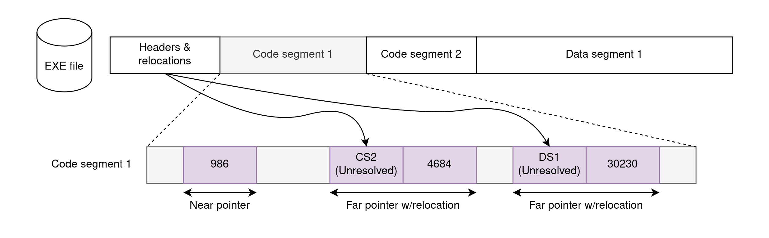
How many segments go into the EXE though? Well, it depends, because not all programs have the same needs. Some programs are tiny overall and could fit in a COM file. Other programs contain large portions of data but little code. Another set of programs contain a lot of code and data. Etc.

So then the question becomes: how can the one-size-fits-all EXE format support these options in an efficient manner? This is where memory models become important, but to talk about those, we must do another detour through pointer types.

Pointer types

The locality principle says that “a processor tends to access the same set of memory locations repetitively over a short period of time”. This is easy to reason about: code normally runs almost-sequentially and data is often packed in consecutive chunks of memory like arrays or structs.

Because of this, expressing all memory addresses as 4-byte segment:offset pairs would be wasteful, and this is where 8086’s segmentation plays in our favor again. We can first load a segment register with the base address of “all of our data” and then all we need to do is record addresses as offsets within that segment. The fewer times we have to reload segment registers, the better because the less information we have to carry around in every instruction and in every memory reference.

But we can’t just always use offsets within a single segment because we may be dealing with more than one segment. And offsets come in various sizes so using a unique size for them all would be wasteful too. Which means memory addresses, or pointers, need to have different shapes and forms, each best suited for a specific use case.

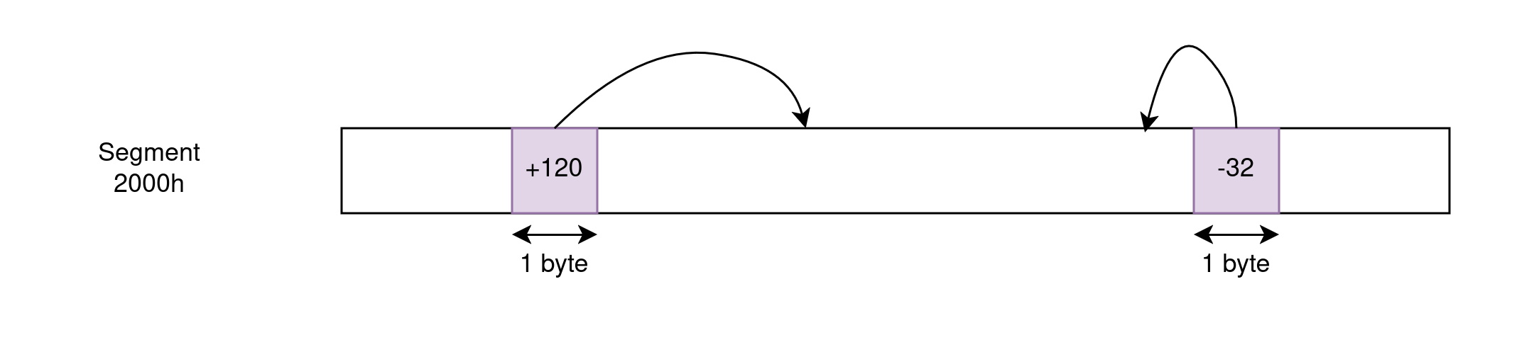
Short pointers take just 1 byte and express a relative address from the instruction being executed. These are specially useful in jump instructions to keep their binary representation compact: jumps appear in every conditional or loop, and in many cases, conditional branches and loop bodies are so short that minimizing the amount of code required to express these branch points is worthwhile.

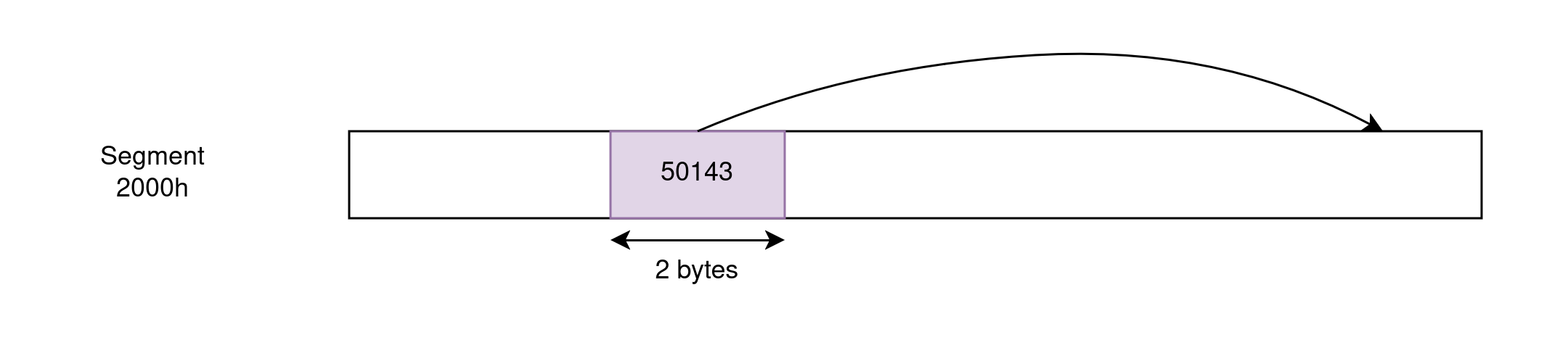
Near pointers can reference addresses within the 64KB segment implied “by context” and are 2-byte long. For example, an instruction like JMP 12829h does not usually need to carry information about the segment this address references because code jumps are almost-always within the same CS of the code issuing the jump. Similarly, an instruction like MOV AX, [5610h] assumes that the given address references the currently-selected DS so that it doesn’t have to express the segment every time. The offset encoded by the near pointer can be relative or absolute.

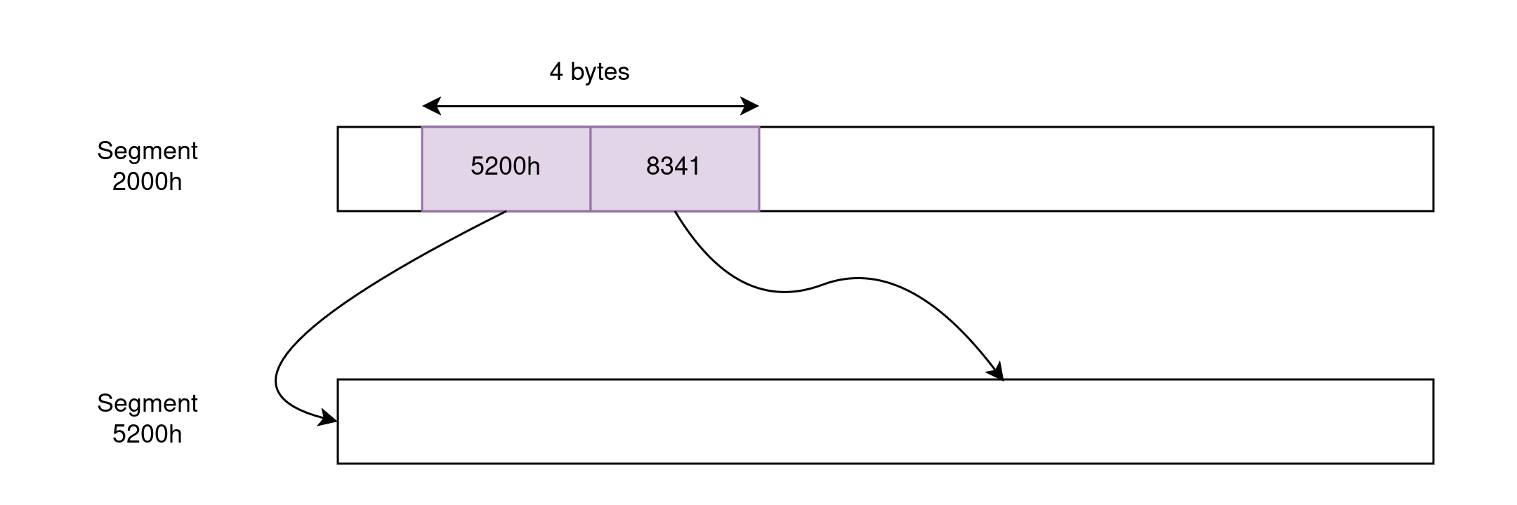
Far pointers can reference any memory address by encoding a segment and an offset. They are 4-byte long. When used in pointer arithmetic, the segment stays fixed and only the offset varies. This is relevant, for example, when iterating over arrays as we can load the base address into DS or ES just once and then manipulate the offset within the segment. However, this means that such iteration has a maximum range of 64KB.

Huge pointers are like far pointers in that they are also 4-byte long and can reference any memory address, but they eliminate the 64KB limitations around pointer arithmetic. They do so by recomputing the segment and offset portions on every memory access (remember that segments are overlapping so we can come up with multiple segment/offset pairs for any physical address). As you can imagine, this requires extra code on every memory access and thus huge pointers impose a noticeable tax on run time.

Memory models

And now that we know about 8086 segmentation, EXE files, and pointer types… we can finally tie all of these concepts together to demystify the memory models we used to see in old compilers for DOS.

Here is the breakdown:

• Tiny: This is the memory model of COM images. The whole program fits in one 64KB segment and all segment registers are set to this one segment at startup. This means that all pointers within the program are short or near because they always reference this same 64KB segment.

• Small: Uses near pointers everywhere, but the data and stack segments are different from the code segment. This means that these programs have 64KB for code and 64KB for data.

• Compact: Uses short pointers for the code but far pointers for the data. This means that these programs can use the full 1 MB memory space for data and, as such, it was particularly useful for games where the code would be as tight as possible while being able to load and reference all assets in memory.

• Medium: The opposite from compact. Uses far pointers for code and short pointers for data. This model is weird because, if you had a program with a lot of code, it was probably the kind of program that handled a lot of data too.

• Large: Uses far pointers everywhere so both code and data can reference the full 1 MB address space. However, because of what far pointers are, all memory offsets are 64 KB at most which means data structures and arrays are limited in size.

• Huge: Uses huge pointers everywhere. This overcomes the limitations of the large model by emitting code to compute the absolute addresses of every memory access and allows structs and arrays that span over 64 KB of memory. Obviously, this comes at a cost: the program code is now larger and the runtime cost is much bigger.

And that’s it!

It is worth highlighting that these models were all conventions that a vintage C compiler used to emit code. If you were writing assembly by hand, you could mix-and-match pointer types to do whatever you wanted given that these concepts had no special meaning to the OS.

Evolving to today’s world

Everything I have told you about until now is legacy stuff that you could easily dismiss as useless knowledge. Or could you?

One thing I did not touch upon is the concept of code density and how it relates to performance. The way we choose to express pointers in the code has a direct impact on code density, so when we evolve computing from 16-bit machines like the 8086 to contemporary 64-bit machines, pointer representations grow by a lot and we face some hard choices.

But to explain all of this and answer the performance questions, you’ll have to wait for the next article. So subscribe now to not miss out on that one!